QunaSys Tech Blog

For the past few years, we have witnessed the advent of near-term quantum computers, or noisy intermediate-scale quantum (NISQ) devices [1]. NISQ devices consist of several tens or hundreds of qubits that are not equipped with error correction and are prone to noise. Owing to these reasons, NISQ devices are not suitable for performing complicated quantum algorithms such as Shor’s algorithm for prime factorization. However, they still allow us to tackle problems that cannot be handled by classical computers and have been extensively studied by both researchers in academia and those in commercial companies.

One of the promising “killer applications” of NISQ devices can be found in the field of quantum chemistry and condensed matter physics, where researchers try to reveal the nature of molecules and solid materials based on quantum mechanics. While calculations by classical computers become exponentially time-consuming as the size of a target system increases, quantum computers can handle the system only in a polynomial amount of computational resources. This unique characteristic of quantum computers (and NISQ devices) attracts a lot of attention from the field of material research for various industrial purposes such as the development of batteries and organic electro-luminescence molecules.

Although a lot of methods have been developed aiming to leverage NISQ devices in investigating quantum systems, there has still been one missing building block: the Green’s function (GF). GF is a cornerstone to understanding quantum systems and tells us a variety of properties of them. For example, GF informs us of what kinds of excitations are present in the target system, which is the clue to predict how the system responds to an external field such as electric field and heat. Despite its importance, however, the NISQ-friendly methods for calculating GF had barely been developed before Ref. [2].

In Ref. [2], methods for calculating Green’s function on near-term quantum computers were proposed by Suguru Endo, Iori Kurata (former interns at QunaSys Inc.), and Yuya O. Nakagawa (Lead researcher at QunaSys Inc.). In that work, two different approaches were proposed. The first approach makes use of the variational quantum simulation (VQS) algorithms [3] to calculate GF directly, while the second approach adopts the so-called Lehmann representation of GF with the subspace-search variational quantum eigensolver (SSVQE) [4] or the multistate-contracted variational quantum eigensolver (MCVQE) [5].

Let us introduce a definition of GF (in the simplest form)

where $H$ is the Hamiltonian of the system, $c_i$ ($c_i^\dagger)$ is the annihilation (creation) operator of electrons at site $i$, and $\ket{G}$ is the ground state of the system.

For a given initial state $\ket{\phi}$ and an ansatz quantum circuit $U(θ)$ (realized on NISQ devices), the original VQS algorithm finds optimal parameters $θ^*$ such that $U(θ^*)\ket{\phi}$ becomes the closest to the time-evolved state $e^{-iHt}\ket{\phi}$. Naive application of the original VQS to the calculation of GF requires the circuit depicted in Fig. 1. This circuit contains two controlled-$U$ gates that should be very complicated and are not expected to run on NISQ devices.

The authors of Ref. [2] extended VQS such that $U(θ^*)\ket{\phi}$ and $U(θ^*)P\ket{\phi}$ simultaneously approximate $e^{-iHt}\ket{\phi}$ and $e^{-iHt}P\ket{\phi}$, where $P$ is some Pauli-gate. The quantum circuit to evaluate GF by using the extended VQS technique is shown in Fig. 2. A variational circuit $U(θ(t))$ which simultaneously approximates the time evolution operator for the initial states $\ket{G}$ and $P_j\ket{G}$ is constructed, instead of two different controlled-unitary operations. This circuit may be feasible on NISQ devices.

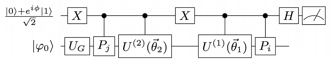
Fig. 1. The direct approach to calculate GS by the VQS algorithm. The upper and the lower horizontal lines represent the ancillary qubit and the qubits for the system of interest. The ground state is generated as |GS〉=U_G|φ_0〉. When Φ=0 (π/2), the real (imaginary) part of GF is evaluated. Adapted from Ref. [2]. For the details, please refer to Fig. 1. of Ref. [2].

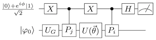
Fig. 2. The extension of the VQS algorithm indicated in FIg. 1. Again, the upper and the lower horizontal lines represent the ancillary qubit and the qubits for the system of interest. $U(θ)$ is the parametrized unitary circuit. Adapted from Ref. [2]. For the details, please refer to Fig. 2. of Ref. [2].

On the other hand, when we calculate GF by the second approach based on SSVQE or MCVQE, we utilize the spectral function representation of GF, or the Fourier transform of GF, defined as

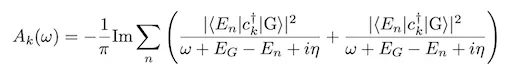
where $E_G$ is the energy of the ground state and $E_n$ is the $n$-th excited state.

SSVQE and MCVQE yield energies of the ground state and excited states as well as their transition amplitudes $\left|\bra{E_n} c_k^\dagger \ket{G}\right|$, $\left|\bra{E_n} c_k \ket{G}\right|$, so simply plugging in those values obtained by SSVQE and MCVQE into the equation above is enough to calculate the spectral function representation of GF.

The authors also provided the resource estimation to calculate GF of the two-dimensional Hubbard model of 25 sites, which is almost impossible to solve exactly by classical computers. According to the estimation, the acceptable fidelity of two-qubit gate operations is 0.1% to calculate GF with the method based on VQS (the first approach) under some assumptions. This value of the fidelity is within the reach of the state-of-the-art NISQ devices [6].

In summary, the methods for calculating GF on near-term quantum computers were proposed by researchers at QunaSys Inc. and collaborators. Since GF is vital to exploring quantum systems, various applications of the methods are expected. For example, they can be used as the solver for the hybrid approach of dynamical mean-field theory [7] or slave boson methods [8] for strongly correlated systems, which are notoriously difficult to be tackled with classical computers. The methods to calculate GF on NISQ devices will broaden our horizon of quantum computing and consequently engineering applications, widening our understandings of more complicated electron systems.

Written by Reika Fujimura and Yuya O. Nakagawa.

[1] J. Preskill, “Quantum Computing in the NISQ era and beyond”, Quantum 2, 79 (2018).

[2] S. Endo, I. Kurata, and Y. O. Nakagawa, “Calculation of the Green’s function on near-term quantum computers” , Phys. Rev. Research 2, 033281 (2020).

[3] Y. Li and S. C. Benjamin, “Efficient Variational Quantum Simulator Incorporating Active Error Minimization”, Phys. Rev. X 7, 021050 (2017).

[4] K. M. Nakanishi, K. Mitarai, and K. Fujii, “Subspace-search variational quantum eigensolver for excited states”, Phys. Rev. Research 1, 033062 (2019). See also this blog post.

[5] R. Parrish et al., “Quantum Computation of Electronic Transitions Using a Variational Quantum Eigensolver”, Phys. Rev. Lett. 122, 230401 (2019).

[6] F. Arute et al., “Quantum supremacy using a programmable superconducting processor”, Nature 574, 505–510 (2019).

[7] B. Bauer et al., “Hybrid Quantum-Classical Approach to Correlated Materials”, Phys. Rev. X 6, 031045 (2016).

[8] Y. Yao et al., “Gutzwiller Hybrid Quantum-Classical Computing Approach for Correlated Materials”, Phys. Rev. Research 3, 013184 (2021).

QunaSys keeps developing efficient quantum algorithms to accelerate various applications of quantum computers. Our mission is to enthusiastically develop technologies that bring out the maximum potential of quantum computers and to continually deliver innovations to society.