Accelerating variational quantum algorithms — A novel way to estimate expectation values on quantum computers

Estimation of expectation values is a key ingredient in variational quantum algorithms [1], regarded as promising candidates for industrial applications of near-term quantum computers. A challenge in the standard ways of expectation value estimation is the necessity to repeat measurement many times to suppress statistical fluctuation, especially in the application to quantum chemistry, which typically demands high accuracy. We proposed [2] an alternative method to estimate the expectation values, which can be more efficient for a certain type of quantum state, frequently encountered in systems of quantum chemistry and condensed matter physics.

The development of Noisy Intermediate-Scale Quantum (NISQ) devices has been rapidly progressing in recent years. Promising applications of NISQ devices are variational quantum algorithms, in particular Variational Quantum Eigensolver (VQE) [3]. VQE can be used to obtain approximations to the lowest energy and the corresponding quantum state (ground state) for electrons in an atom or a molecule and can be applied to quantum chemistry, condensed matter physics, etc.

VQE is a hybrid quantum-classical algorithm based on the variational method: for a given trial wavefunction and Hamiltonian (the quantum-mechanical operator for energy) of some physical system of interest, quantum computers are used to estimate the energy expectation value; the latter is minimized with respect to parameters describing the trial wavefunction by use of a classical computer; this enables us to iteratively find the approximate lowest-energy state within a set of states described by the trial wavefunction. In this algorithm, the task for quantum computers is to estimate the expectation value. To do so, the trial wavefunction is prepared as a quantum circuit, for which “energy” is measured, and such a set of preparation-measurement procedures is repeatedly performed for statistical estimation. Since the number of measurements is finite, the estimated expectation value is inevitably accompanied by statistical fluctuation. It is highly desirable to suppress the amount of statistical fluctuation with as few measurements as possible in order to perform VQE calculations with high precision and efficiency.

The standard way of expectation value estimation [3] goes like this: firstly, the Hamiltonian is decomposed into quantities that can be measured by NISQ devices (specifically, the quantities are so-called Pauli strings, tensor products of Pauli operators); then, each of these quantities is estimated by measuring a quantum circuit; finally, recombining the estimates of those quantities, the overall estimate of the energy expectation value is obtained. The procedure is rather simple but relies on potentially huge statistical resources: estimating each of Pauli strings requires many measurements to suppress statistical fluctuation; besides, the number of Pauli strings to be measured increases significantly with the system size [4]; then, the total number of measurements can be too huge to finish the expectation value estimation within a practically acceptable time, especially when high accuracy is required as in quantum chemistry. There are vigorous efforts to improve this deficit, e.g., by simultaneously measuring commuting Pauli strings and/or by optimizing the allocation of measurement budget to each of Pauli strings. Yet, further improvements are still awaited toward practical use for systems of industrial interest. (See [5] for a recent assessment of measurement resources in the application to quantum chemistry calculations.)

We pursued another direction in expectation value estimation: instead of decomposing the Hamiltonian into measurable quantities, our method relies on the decomposition of the wave function into computational basis states. Specifically, we express the expectation value of the Hamiltonian $H$ for a wave function $\ket{\psi}$ as

\bra{\psi}H\ket{\psi}\sum_{m,n}|\braket{m|\psi}|^2 |\braket{n|\psi}|^2\dfrac{\bra{m}H\ket{n}}{\braket{m|\psi}\braket{\psi|n}}

where the computational basis states, for $N$ qubits, are labeled by $m, n = 0, 1, …, 2ᴺ -1$ (for details, see Eq. (6) and explanation around it in [2]). Our method is based on the insight that a wave function of interest in quantum chemistry and condensed matter physics can often be well-described by a relatively small number of electron configurations, each of which can be identified as a computational basis state on quantum computers. We call such a state a “concentrated” state in particular computational basis states. With this insight, we approximated the expectation value above as the sum of contributions from those major electron configurations or computational basis states. The major basis states can be selected by sampling the wave function, generated on quantum computers, in the computational basis. The transition matrix elements $\bra{m}H\ket{n}$ can be efficiently calculated by a classical computer, while the remaining pieces in the above equation can be estimated based on quantities measured on quantum computers, each of which requires a quantum circuit consisting of at most $N$ CNOT gates in addition to the ones for the wave function $\ket{\psi}$ . The point is that the number of quantities to be measured is $O(R)$ , where $R$ means the number of the major basis states. Hence, when $R$ is significantly smaller than the number of Pauli strings in the decomposition of the Hamiltonian, our method is expected to be more efficient than the standard methods in terms of statistical convergence.

In order to assess the performance of our method, we took small molecules such as water and methane as an example and considered the expectation value estimation for their electronic Hamiltonian and ground states. Calculating the variance of the energy expectation value for each molecule, we evaluated the number of measurements to suppress the amount of statistical fluctuation below the required accuracy (1 mHartree), which is then compared with the ones evaluated for the standard methods. The result is summarized in the following figures, which include the standard methods with basic implementation (No grouping) and with improvements by grouping mutually commuting Pauli strings (QWC and GC), for two ways of the measurement allocation to each of the measured quantities.

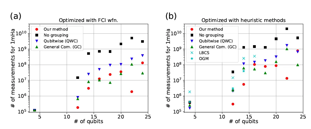
The result tells that (1) the numbers of measurements can be generically reduced by several orders of magnitude in comparison with “No grouping”, (2) our method is generically better than “QWC” (grouping of qubit-wise commuting Pauli strings), (3) our method tends to be comparable with “GC” (grouping of general-commuting Pauli strings). We remark that the GC grouping requires more expensive quantum circuits [6] than our case, i.e., $O(N²)$ (GC) vs. $O(N)$ (ours) extra two-qubit gates in addition to the circuit for the wave function, and hence is more challenging to implement on noisy devices.

In summary, we proposed an alternative way for expectation value estimation, and demonstrated that our method can be more efficient than the standard methods in terms of statistical convergence. Our method can be incorporated in VQE as a subroutine, which may speed up VQE. The method can be applied to expectation value estimation of generic observables, and thus can be used in combination with variational quantum algorithms other than VQE. It is open to a wide range of applications.

References and footnote

[1] For review, see, e.g., Suguru Endo, Zhenyu Cai, Simon C. Benjamin, Xiao Yuan, “Hybrid Quantum-Classical Algorithms and Quantum Error Mitigation”, J. Phys. Soc. Jpn. 90, 032001 (2021). [https://journals.jps.jp/doi/10.7566/JPSJ.90.032001]

[2] M. Kohda, R. Imai, K. Kanno, K. Mitarai, W. Mizukami, and Y. O. Nakagawa, “Quantum expectation value estimation by computational basis sampling”, arXiv:2112.07416. [https://arxiv.org/abs/2112.07416]

[3] Alberto Peruzzo, Jarrod McClean, Peter Shadbolt, Man-Hong Yung, Xiao-Qi Zhou, Peter J. Love, Alán Aspuru-Guzik, and Jeremy L. O’Brien, “A variational eigenvalue solver on a photonic quantum processor”, Nat. Commun. 5, 4213 (2014). [https://www.nature.com/articles/ncomms5213]

[4] For instance, the number of the Pauli strings scales as O(N⁴) for a Hamiltonian of electronic state in a molecule, where N is the number of spin-orbitals or qubits. It is only polynomial in the system size, but can be numerically large, given a nominal target of quantum computations would be N≈100 or beyond.

[5] Jérôme F. Gonthier, Maxwell D. Radin, Corneliu Buda, Eric J. Doskocil, Clena M. Abuan, Jhonathan Romero, “Identifying challenges towards practical quantum advantage through resource estimation: the measurement roadblock in the variational quantum eigensolver”, arXiv:2012.04001. [https://arxiv.org/abs/2012.04001]

[6] Pranav Gokhale, Olivia Angiuli, Yongshan Ding, Kaiwen Gui, Teague Tomesh, Martin Suchara, Margaret Martonosi, Frederic T. Chong, “Minimizing State Preparations in Variational Quantum Eigensolver by Partitioning into Commuting Families”, arXiv:1907.13623. [https://arxiv.org/abs/1907.13623]

Written by Masaya Kohda.