 QunaSys Tech Blog
Quantum-Selected Configuration Interaction (QSCI) uses a quantum device to sample an ansatz state and propose which electronic configurations, or determinants, matter for the state of interest. A classical solver then builds and diagonalizes the Hamiltonian within that selected subspace. The resulting energy is variational: exact within the chosen subspace and improving monotonically as the subspace grows [1, 2]. Larger selected subspaces can therefore improve the result, but only if the classical solver can handle them.
At QunaSys, we are developing a QSCI implementation for QURI SDK Enterprise. Before this work, its classical stage had to build and diagonalize the selected-subspace Hamiltonian on one Message Passing Interface (MPI) rank, limiting problem size to the memory available to one process. We distributed both stages, with each MPI rank holding only part of the matrix. On Fugaku, the new solver reaches four million determinants. At one million determinants, Hamiltonian construction gets 11.8x faster from 4 to 96 ranks. The runs exposed the next bottlenecks: diagonalization dominates at the largest subspaces, and every attempt at eight million determinants ran out of memory during assembly. Hamiltonian density predicted the cost more reliably than qubit count.
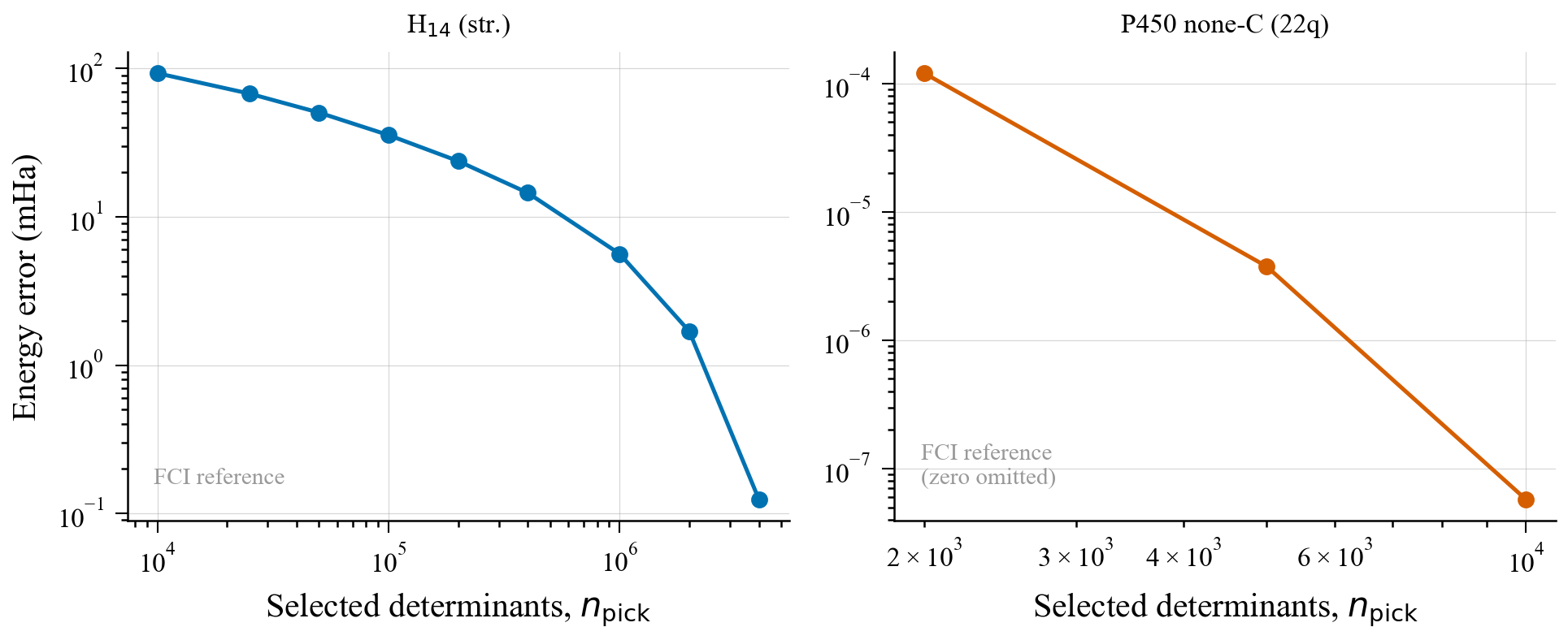
Figure 1. Energy error versus selected determinants at 32 ranks. H14 uses an independently calculated FCI energy as its reference; the bare P450 model uses its computed energy over the complete 18,150-determinant space. The zero-error P450 endpoint is omitted because the vertical axes are logarithmic.
What we benchmarked
The solver is a distributed QSCI implementation developed for QURI SDK Enterprise but not yet included in a release, run on Fugaku. It builds the truncated Hamiltonian row-partitioned across ranks, so no single rank ever holds the whole matrix, and hands it to PETSc for distributed matrix storage and SLEPc for a distributed Krylov-Schur solve [3, 4].
All runs are on Fujitsu A64FX nodes [5], 48 cores per node and 32 GiB of high-bandwidth memory (HBM2), with OMP_NUM_THREADS=1 throughout. Ranks are spread thin for memory reasons the next sections make concrete. The fixed-32-rank runs, including every four-million-determinant point, use one rank per node: 32 whole nodes, each rank backed by a full node's 32 GiB. Those fixed-size runs are distinct from the strong-scaling sweep. For 4-to-16-rank jobs we use one rank per node and for 32-to-96-rank jobs four ranks per node. The 96-rank strong-scaling runs therefore use 24 nodes. At one million determinants H18 needs about 4 nodes’ whole memory.
We measured nine systems. Four stretched linear hydrogen chains, H14, H18, H20 and H22, span 28 to 44 qubits and provide a strongly correlated, comparatively sparse stress case. Four models of a cytochrome P450 active site span 22 to 30 qubits and provide denser, realistic chemistry; they differ in the axial ligand. Water in a 6-31G basis is the fully characterised control. We report the sparse and dense families separately because Hamiltonian density matters more than qubit count.
Our determinant sets come from full configuration interaction or heat-bath configuration interaction (HCI) [2], rather than uniform random sampling. HCI ranks determinants by an estimated importance criterion and favors strongly coupled configurations, making these subspaces demanding inputs for matrix construction and diagonalization. No quantum sampling fed the runs below. This isolates the solver's performance on determinant sets of known provenance from the sampler's statistics.
Throughout, we split the classical step into H-build, assembling the truncated Hamiltonian, and diag, diagonalizing it, against subspace size as the independent variable. Each QSCI invocation records two timed repetitions, and we report the repetition with the shortest total time. The repetitions share one allocation rather than repeating the whole job, so treat the resulting ratios as point estimates. The SBD comparison later in the post has one measurement per point.
Where the time actually goes
| System | Ranks | Determinants | H-build | Diag | Diag share |
|---|---|---|---|---|---|
| H14 | 32 | 10K | 0.14 s | 0.05 s | 25% |
| H14 | 32 | 1M | 13.4 s | 35.5 s | 73% |
| H14 | 32 | 4M | 101.3 s | 376.7 s | 79% |
| H18 | 32 | 100K | 1.2 s | 0.9 s | 42% |
| H18 | 32 | 1M | 16.0 s | 31.3 s | 66% |
| P450 (oxo) | 32 | 100K | 1.5 s | 3.4 s | 69% |
| H2O | 32 | 200K | 1.5 s | 3.6 s | 71% |
On H14, diag's share climbs from 25% at ten thousand determinants to 79% at four million. Among the hydrogen chains, it becomes the majority cost at 100K determinants for H14, 400K for H18 and H20, and one million for H22. It dominates at the largest subspace measured for every system. The measurements shifted our optimization target from matrix assembly to diagonalization.
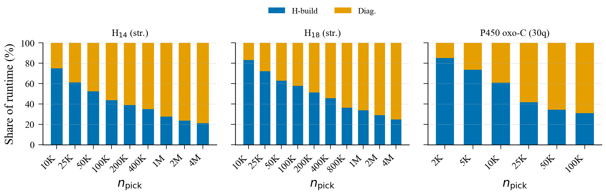
Figure 2. H-build and diag shares versus subspace size at 32 ranks for two hydrogen chains and the P450 oxo model.
Hamiltonian density is an independent axis
Compare the two 100K rows above: H18 is a 36-qubit sparse chain and diagonalizes in 0.9 s, while the 30-qubit P450 oxo model takes 3.4 s at the same rank count and subspace size. Fewer qubits, nearly four times the cost, because the Hamiltonian is denser.
Strong scaling
H-build scales 11.8x from 4 to 96 ranks on our reference case, H18 at one million determinants: 90.9 s down to 7.7 s across a 24x increase in ranks. H-build was still scaling at 96 ranks, the largest rank count we tested. The curve crosses two configurations: the 4-to-16-rank jobs give each rank a whole node, while the 32-to-96-rank jobs place four ranks on each node. It therefore reports the elapsed time of the configurations we ran, not a uniform-layout scaling study.
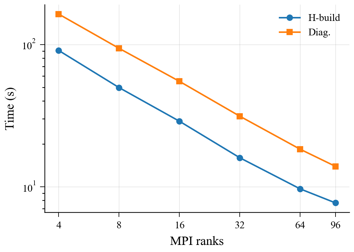
Figure 3. H-build and diag wall-clock time versus rank count, H18 at one million determinants. The layout changes from one rank per node through 16 ranks to four ranks per node from 32 ranks onward.
Diagonalization scales almost identically: 11.8x over the same 4-to-96-rank range, 163.8 s down to 13.9 s. Fitting T = T_s + T_p/P across the full 4-to-96-rank series puts the serial fraction at 2.0% for H-build and 3.4% for diag. So the two phases do not differ in how well they parallelize; they differ in absolute cost, and diag is roughly twice H-build's at every rank count we measured. The classical step is diag-bound because diag is bigger, not because it scales worse.
This campaign isolates Hamiltonian construction and diagonalization; sampling performance is outside its scope.
Scaling beyond four million
With 32 MPI processes, each process stored about 0.5 GiB of coordinate arrays at one million determinants, 1.2 GiB at two million, and 3.0 GiB at four million. Nonzero counts, recorded directly, grow as dim^1.32 to dim^1.39 depending on the system, measured across 10K to 4M determinants with R-squared values of 0.995 or higher. Per-rank memory grows more slowly than that because load balance improves with subspace size: across the four chains, the heaviest rank holds 2.4x to 2.9x its even share at 25K determinants and 1.3x to 2.2x at four million. The matrix itself carries a flat 16 bytes per nonzero, from 32-bit indices and 64-bit reals.
Those figures are the matrix in coordinate form, a floor rather than the requirement. During assembly, the coordinate arrays, the compressed structure PETSc builds from them, and PETSc's coordinate index map can all be resident at once. Byte accounting estimates that transient at about 2.7 times the recorded coordinate-array footprint. Fugaku's process-level memory counter did not capture these allocations, so this multiplier is an estimate rather than a direct peak-memory measurement. The eigensolver's Krylov basis adds tens of megabytes per rank, which is not the binding term. Applying the estimate to the measured four-million-determinant footprint gives about 8 GiB per rank. A node's memory does not divide by its core count at all here: those runs give one rank an entire 48-core node, using a little over a quarter of its memory and a single one of its cores, purely to have somewhere to put the matrix.
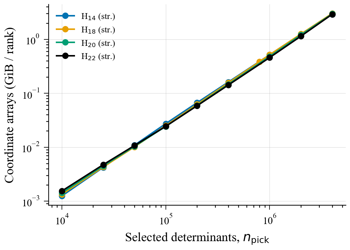
Figure 4. Measured per-rank coordinate-array footprint versus subspace size for the four hydrogen chains.
By pushing to eight million determinants, we isolated assembly as the next target. Every chain we tried ran out of memory during assembly even though the steady-state footprint would fit.
It would be convenient to call this a soft limit, on the grounds that memory per rank recedes as nodes are added. Our own weak-scaling numbers do not support that reading. Holding determinants-per-rank fixed at 25,000 and growing the job from 1 to 96 ranks, H-build time grows 4.8x, per-rank memory grows 13.4x, and diag time grows 34x. Adding nodes to hold a larger subspace therefore does not deliver that subspace at constant time to solution. It converts a memory wall into a time wall a short distance behind it.
Adding capacity alone does not buy problem size; not forming the matrix in the first place does. A matrix-free operator application avoids both the peak memory use during assembly and the steady-state matrix footprint, and it is the same code path the eigensolver work has to go through anyway.
Comparison against a reference implementation
We ran the same problems against Selected Basis Diagonalization (SBD), the eigensolver used in the qiskit-community/qiskit-c-api-demo implementation of Sample-based Quantum Diagonalization (SQD) [6, 8]. SQD is a QSCI-based workflow augmented with configuration recovery and related post-processing. This benchmark therefore compares two implementations of the classical selected-subspace diagonalization step at approximately matched subspace dimensions. Both sides ran at the same rank count with OMP_NUM_THREADS=1, with timings excluding Hamiltonian file I/O and setup.
Our solver is faster at every P450 subspace we tested. At 2,000 determinants it is 1.8x to 3.5x faster; at the largest subspace for each model, the margin is 8.5x for the water ligand, 11.5x for oxo, 16.9x for pyridine and 15.5x for the bare model, whose 18,150 determinants span its entire CI space.
Both sides start from complete FCI-ranked determinant pools, but they construct a subspace differently. QSCI keeps the highest-ranked alpha-beta determinant pairs as a flat list, while the bridge to SBD ranks alpha and beta strings separately and diagonalizes their Cartesian product. At 100,000 determinants, the two spaces overlap by 58% for the water ligand and 47% for pyridine and oxo. Only the bare model reaches its full 18,150-determinant CI space, where the two matrices are identical. Across all 22 P450 points the two energies differ by at most 0.36 mHa, and by under 0.01 mHa at every subspace of 25,000 determinants or more. The timing ratios therefore compare different subspaces of approximately the same dimension that produce closely agreeing energies, not identical matrices except at the bare model's full-space point.
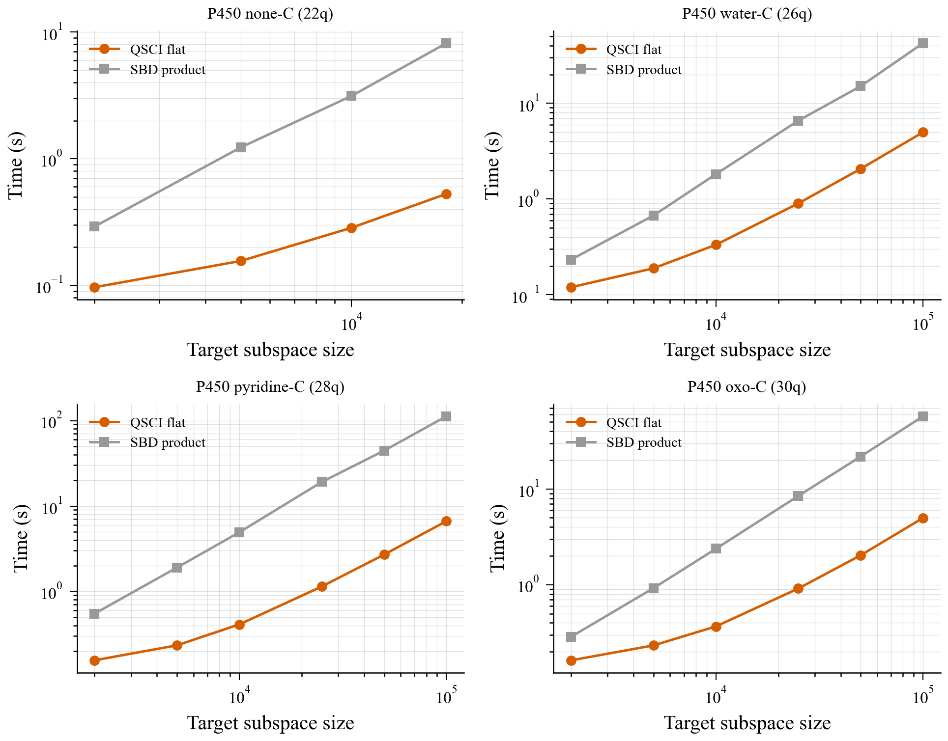
Figure 5. QSCI and SBD wall-clock time versus target subspace size for the four P450 models at 32 ranks. Dimensions are approximately matched; the determinant sets differ except at the full-space endpoint.
Benchmark conditions
-
Implementation. Our comparison target is the CPU implementation in
qiskit-c-api-demoat commit47dbfb7, with SBD submodule commitf0b85ad[8]. We applied a local benchmark patch to run precomputed subspaces, accept separate alpha and beta determinant files, and record split timings. The patch is available on request. A GPU-accelerated variant of SBD exists [7]; our runs are CPU-only on A64FX, so that comparison is outside the scope of this campaign. - Optimization. Our implementation was actively profiled over the course of this campaign; SBD was not tuned to a comparable degree. If it has headroom similar to what we found in our own code, these margins would narrow.
-
SBD settings. Its time limit defaults to 600 s and can return an unfinished result without signalling one, so we set it to 7,200 s for the P450 sweep. We also set the iteration cap to 200, the block size to 40 and the tolerance to
1e-9; block size 40 was roughly twice as fast as the default of 10 at large subspace sizes. -
Tolerances. Eigensolver tolerances are not exactly matched: SLEPc's default
1e-8tolerance and SBD's tighter1e-9tolerance. In separate four-rank controls, rerunning QSCI at1e-9increased diagonalization time by 4% to 14% across H18 and two P450 cases, with no meaningful change in energy. The largest observed change was a factor of 1.14, compared with the reported factors of 8.5 to 16.9.
Correctness on a near-degenerate case
On water in a 6-31G basis, our SLEPc solve returns -76.1208 Ha from a flat subspace of 200,000 determinants. SBD instead diagonalizes a 447-by-447 product containing 199,809 determinants and returns -74.108 Ha. The complete fixed-particle-number CI space contains 1,656,369 determinants, so the 447-by-447 product is only a selected subspace, not the entire CI space. The two subspaces share 55,693 determinants, about 28%, so the QSCI energy is not a variational bound on SBD's matrix.
SBD's product does contain the Hartree-Fock determinant, whose energy for this Hamiltonian is -75.984 Ha. The lowest eigenvalue in that subspace cannot be higher than the expectation value of a determinant it contains. SBD's result is 1.88 Ha above that bound, so it cannot be the lowest eigenvalue of its own matrix.
SBD stops after 15 of the allowed 200 iterations, reports a residual of 4.7e-10 against the requested 1e-9, and exits successfully. By its own criterion it has converged, but not to the ground state. Raising the iteration cap from 200 to 2,000 does not change any reported digit. Increasing the Davidson block size or loosening the tolerance produces different energies, all above the Hartree-Fock bound. Those settings do not change the matrix or its ground-state energy.
SBD hard-codes its initial guess and exposes no preconditioner, so neither remedy could be tested. Because SBD does not return the correct ground-state energy, there is no valid SBD runtime to compare.
Where this goes next
Our next implementation target is a matrix-free eigensolver. It addresses both constraints exposed here: diagonalization consumes most of the runtime at the largest subspaces, while materializing the Hamiltonian pushes peak memory high enough to stop the calculation at eight million. Removing that matrix would also let us use more of each node's compute capacity instead of allocating whole nodes mainly for memory.
The practical benefit is access to selected subspaces beyond a single process's capacity limit. Because these benchmarks used determinants from full configuration interaction or HCI rather than quantum sampling, the next campaign will connect that engineering result to chemistry by pairing the matrix-free solver with determinants sampled from quantum hardware and comparing accuracy and cost against HCI, density matrix renormalization group (DMRG), and coupled cluster on a strongly correlated target.
Software and versions:
-
QURI SDK Enterprise revision
8314ff0 - Python 3.11.11
- PETSc 3.24.5
- SLEPc 3.24.2
-
qiskit-c-api-democommit47dbfb7 -
SBD commit
f0b85ad.
Acknowledgements
This work used computational resources of the supercomputer Fugaku provided by RIKEN Center for Computational Science (Project hp260359).
References
- K. Kanno, M. Kohda, R. Imai, S. Koh, K. Mitarai, W. Mizukami, Y. O. Nakagawa. Quantum-selected configuration interaction: classical diagonalization of Hamiltonians in subspaces selected by quantum computers. Phys. Rev. Research 8, 023268 (2026). https://doi.org/10.1103/dmn4-snfx.
- A. A. Holmes, N. M. Tubman, C. J. Umrigar. Heat-bath configuration interaction: an efficient selected configuration interaction algorithm inspired by heat-bath sampling. J. Chem. Theory Comput. 12(8), 3674-3680 (2016). https://doi.org/10.1021/acs.jctc.6b00407.
- S. Balay et al. PETSc/TAO Users Manual. Argonne National Laboratory, ANL-21/39, Revision 3.24.
- V. Hernandez, J. E. Roman, V. Vidal. SLEPc: a scalable and flexible toolkit for the solution of eigenvalue problems. ACM Trans. Math. Software 31(3), 351-362 (2005). https://doi.org/10.1145/1089014.1089019.
- M. Sato et al. Co-design for A64FX manycore processor and Fugaku. SC20: International Conference for High Performance Computing, Networking, Storage and Analysis (2020). https://doi.org/10.1109/SC41405.2020.00051.
- J. Robledo-Moreno et al. Chemistry beyond the scale of exact diagonalization on a quantum-centric supercomputer. Sci. Adv. 11, eadu9991 (2025). https://doi.org/10.1126/sciadv.adu9991.
- J. Doi, T. Shirakawa, Y. Kawashima, S. Yunoki, H. Horii. GPU-accelerated selected basis diagonalization with Thrust for SQD-based algorithms. arXiv:2601.16637 (2026).
-
qiskit-community.
qiskit-c-api-demo. GitHub, commit47dbfb70c785fc5465ac60f737e4899318e96741, withr-ccs-cms/sbdcommitf0b85ada8f8ad76e123d9e1ad4ed7d769dd08518. https://github.com/qiskit-community/qiskit-c-api-demo/tree/47dbfb70c785fc5465ac60f737e4899318e96741