Concrete Quantum Resource Estimation for Quantitative Finance — Solving the Black–Scholes Equation with LCHS

One promising application of quantum computers is quantitative finance. Quantitative finance involves a variety of mathematical frameworks depending on the target problem, and partial differential equations (PDEs) are one such framework. PDEs also frequently appear in fields known as CAE (Computer-Aided Engineering), such as fluid dynamics and structural analysis, and many approaches have been proposed for solving or accelerating them with quantum computers (see our tech-blog post).

In this article, we introduce a quantum circuit implementation and resource estimation using QURI SDK for the Black–Scholes equation, a PDE used in a canonical quantitative-finance problem: option pricing. More specifically, we discretize the Black–Scholes equation using the finite difference method, design and simulate a quantum circuit that computes the solution using a method called LCHS (Linear Combination of Hamiltonian Simulation), and estimate the required computational resources.

Note: To keep the article concise, some technical details are omitted. Please refer to the references for further details.

Quantitative finance

Quantitative finance is a field that treats pricing of financial derivatives, risk management, investment decisions, and so on. Typical problems include:

How to model changes in asset prices — representing how stock prices, interest rates, exchange rates, and similar quantities evolve over time using mathematical formulas
How to evaluate financial derivatives at a “fair price” — determining the price of a contract that depends on an underlying asset, such as a stock
How to manage and optimize risk — deciding how to choose a portfolio of assets and how to measure the risk of loss

Corresponding to these problems, different mathematical frameworks are used, such as stochastic differential equations for asset price models, partial differential equations for pricing equations, and optimization problems for portfolio optimization.

The “option” considered in this article is a type of financial derivative that gives the holder the right to buy or sell an underlying asset, such as a stock, at a predetermined price, called the strike price $K$ , at a predetermined future time, called the maturity $T$ . Depending on when the option can be exercised, options are classified into types such as European options, which can be exercised only at maturity, and American options, which can be exercised at any time up to maturity.

Below, we consider a European call option, which is the right to buy. If the underlying asset price at maturity is $S_T$ , then when $S_T>K$ the holder can exercise the right and obtain a profit of $S_T-K$ . When $S_T\le K$ , the holder can simply abandon the option. Therefore, the value at maturity $T$ is expressed as $\max(S_T-K,0)$ . The goal is to evaluate the present value of this option.

The Black–Scholes equation

As the simplest asset price model, assume that the underlying asset price $S_t$ at time $t$ follows geometric Brownian motion:

dS_t = \mu S_t\, dt + \sigma S_t\, dW_t

Here, $W_t$ is standard Brownian motion, while $\mu$ and $\sigma$ are constants called the drift and volatility, respectively. Under assumptions such as a frictionless market with no transaction costs and the no-arbitrage condition that there are no trading opportunities that guarantee profit without risk, the option price $V(S,t)$ when the underlying asset price is $S$ at time $t$ satisfies the following PDE:

\frac{\partial V}{\partial t} + \frac{1}{2}\sigma^2S^2\frac{\partial^2V}{\partial S^2} + rS\frac{\partial V}{\partial S} - rV = 0

Here, $r$ is the risk-free interest rate. The terminal condition is $V(S,T)=\max(S-K,0)$ . This is the one-asset Black–Scholes equation, which can be extended to multi-asset cases by considering multiple underlying assets.

For the one-asset case, the following analytical solution is known:

V(S,t) = S\,\Phi(d_1) - Ke^{-r(T-t)}\,\Phi(d_2) \\ d_1 = \frac{\ln(S/K)+\left(r+\frac{1}{2}\sigma^2\right)(T-t)}{\sigma\sqrt{T-t}}\, \\ d_2 = d_1-\sigma\sqrt{T-t}

Here, $\Phi$ is the cumulative distribution function of the standard normal distribution. Figure 1 shows the analytical solution $V(S,t)$ for different remaining times to maturity, with parameters $K=60,\sigma=0.2,r=0.03,T=3$ . As maturity $T$ approaches, the analytical solution approaches the payoff at maturity, $\max(S-K,0)$ , shown by the dashed line. In general, analytical solutions do not exist for multi-asset cases, so numerical computation is required.

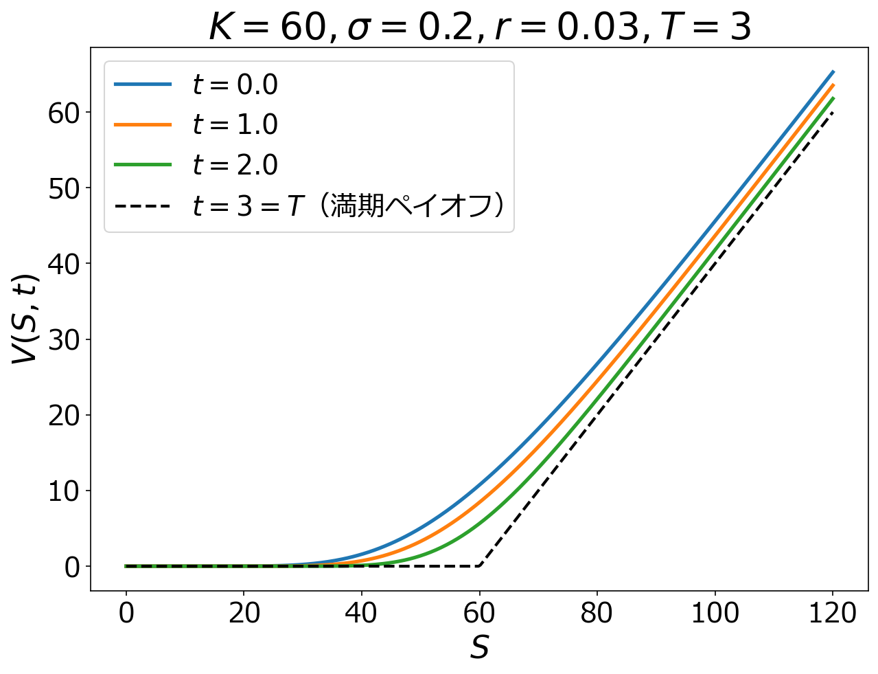
Figure 1: Analytical solution of the one-asset Black–Scholes equation

Boundary conditions

To determine the solution, boundary conditions must be given at both ends, $S\to 0$ and $S\to\infty$ . At $S=0$ , the option value is identically $0$ , so $V(0,t)=0$ . On the other hand, as $S\to\infty$ , a call option becomes approximately equivalent to a contract that will almost certainly be exercised. Under continuously compounded interest rate $r$ , the value $K$ at maturity $T$ corresponds to $Ke^{-r(T-t)}$ at the present time $t$ , so the price is $V(S,t)=S-Ke^{-r(T-t)}$ . In particular, the derivative with respect to $S$ asymptotically approaches $\partial_S V(S,t)=1$ . These behaviors are also consistent with the analytical solution.

Quantum circuit implementation strategy

A linear PDE such as the Black–Scholes equation can be rewritten as an affine map for an $N$ -dimensional vector $\vec{V}(t)$ , whose entries are the values at each grid point at time $t$ , by discretizing the spatial direction — in this case, the underlying asset price $S$ — into $N$ points:

\frac{d\vec{V}(t)}{dt} = A \vec{V}(t) + \vec{b}

Here, $A$ is an $N$ -by- $N$ square matrix and $\vec{b}$ is an $N$ -dimensional vector. The price at maturity $T$ , or payoff, is known, and the quantity we want is the price $\vec{V}(0)$ at the present time. Formally, this can be computed as:

\vec{V}(0) = e^{-AT} \vec{V}(T) - \int_0^T d\tau\, e^{-A\tau} \vec{b}

This form is exactly the same as that of linear PDEs appearing in CAE fields such as fluid and structural analysis, so existing quantum algorithms such as Schrödingerisation can be applied directly [1]. In this study, we adopt a method called LCHS, which implements non-unitary time evolution as a weighted sum of unitary operations.

Quantum circuit implementation using LCHS

Spatial discretization

For a sufficiently large upper bound $S_{\max}$ , we discretize the underlying asset price $S\in[0,S_{\max}]$ into $N$ points, $S_0,\dots,S_{N-1}$ , with spacing $\Delta S$ , and define $V_j(t):=V(S_j,t)$ . Using a central finite difference approximation, the Black–Scholes equation becomes the following system of ordinary differential equations for $j=1,\dots,N-1$ (the argument $t$ is omitted for simplicity):

\frac{dV_j}{dt} = rV_j - \frac{1}{2}\sigma^2 S_j^2 \frac{V_{j+1} - 2V_j + V_{j-1}}{(\Delta S)^2} - r S_j \frac{V_{j+1} - V_{j-1}}{2\Delta S}

At the endpoints, the boundary condition $V(0,t)=0$ allows us to set $V_0=0$ for $j=0$ . At $j=N-1$ , a virtual grid point $V_N$ appears, but from the boundary condition $\lim_{S\to\infty}\partial_S V(S,t)=1$ , we set $V_N=V_{N-2}+2\Delta S$ .

Let the vector of prices at each grid point be:

\vec{V}(t) = (V_0(t),\dots,V_{N-1}(t))

By rearranging this equation, we obtain the matrix $A$ and vector $\vec{b}$ . The terminal values are $V_j(T)=\max(S_j-K,0)$ .

LCHS

The matrix $A$ is generally not anti-Hermitian, and the time evolution $e^{-At}$ above is non-unitary. Quantum computers, however, naturally implement unitary transformations. Therefore, additional techniques are needed to compute non-unitary time evolution.

LCHS (Linear Combination of Hamiltonian Simulation) is a method that represents non-unitary time evolution $e^{-At}$ as a weighted integral of unitary time evolutions $e^{-i(kL+H)t}$ :

e^{-At} = \frac{1}{\sqrt{2\pi}}\int_{\mathbb{R}} dk\; f(k)\, e^{-i(kL+H)t} \approx \frac{1}{\sqrt{2\pi}}\sum_{m=-M}^{M} \Delta k\, f(k_m)\, e^{-i(k_mL+H)t} \quad \quad (1)

Here:

$f(k)$ is called a kernel function.
The number of partitions is $2M+1$ , the width is $\Delta k$ , and the representative point of each partition is $k_m=m\Delta k$ .
$L=(A+A^\dagger)/2$ and $H=(A-A^\dagger)/(2i)$ are both Hermitian matrices.

Each $e^{-i(kL+H)t}$ can be implemented using QSVT (Quantum Singular Value Transformation), while the summation over $k$ can be implemented using LCU (Linear Combination of Unitaries). QSVT uses a quantum circuit that embeds an arbitrary matrix, not necessarily unitary, as a submatrix, and realizes a new quantum circuit that embeds various polynomial transformations of the matrix’s eigenvalues or singular values. Here, we realize the unitary time evolution $e^{-i(kL+H)t}$ by approximating $e^{-ixt}$ with a finite-degree polynomial in $x$ [2].

The kernel function $f(k)$ must satisfy several mathematical constraints. Here, we use the function proposed by Low and Somma [3]:

f(k;\gamma)= \sqrt{\frac{2}{\pi}} \frac{e^{1-ik}}{1+k^2} \exp\left(-\frac{k^2+1}{4\gamma^2}\right)

Here, $\gamma$ is a real number chosen according to the allowed error.

In simulations using LCHS, errors arise both from making the integration interval finite and discretizing it in Equation (1), which is the error of LCHS itself, and from approximating $e^{-ixt}$ by a finite-degree polynomial in QSVT. In actual simulations, the partitions and polynomial degree must be chosen appropriately according to the allowed error of the overall solution.

LCHS also requires realizing the Hermitian matrices $L$ and $H$ as quantum circuits. For example, in this case, the diagonal element $(j,j)$ of $L$ is given as a polynomial in $j$ , such as $r+\sigma^2j^2$ . In this study, we implement and compare two approaches: Encoding A, which classically computes this polynomial and implements the corresponding components using multi-controlled gates, and Encoding B, which computes the polynomial on a quantum circuit.

Scaling and quantum advantage

Let the number of grid points be $N=2^n$ , and consider costs that depend on the number of grid points. Omitting the details, the number of gates required to embed each matrix $L,H$ into a quantum circuit is $O(2^n)$ for Encoding A and $O(n)$ for Encoding B; the trade-off is that Encoding B requires more auxiliary qubits. In the following, unless otherwise stated, we assume the gate-efficient Encoding B. Because the equation contains a second-derivative term, the norm of the matrix $A$ scales as $\|A\|\sim O(1/(\Delta S)^2)\sim O(2^{2n})$ . As a result, the number of QSVT calls increases accordingly, and the number of gates required for time evolution is $O(2^{2n}n)$ .

In actual quantum computation, in addition to the implementation of the time-evolution part described so far, it is necessary to prepare the initial quantum state and read out the computational result.

For the initial state preparation, we prepare a quantum state corresponding to the terminal condition $\vec{V}(T)$ at $t=T$ , embedding the simple piecewise linear function $\max(S-K,0)$ into the amplitudes of the state. This can be achieved with cost $O(n)$ .
By measuring the quantum state obtained after time-evolution simulation using LCHS, we can read out the option price at $t=0$ . Since the typical amplitude of each computational basis state in the final state is $O(1/\sqrt{N})$ , quantum amplitude estimation to obtain a specific $V_j(0)$ is estimated to require $O(2^{n/2})$ operations.

Combining these components, the cost of quantum computation that depends on the number of grid points becomes:

(O(n)+O(2^{2n}n)) \cdot O(2^{n/2}) = O(2^{5n/2}n)

On the other hand, in classical computation, the computational complexity of a matrix exponential $e^{-AT}$ is generally known to be $O(2^{3n})$ when using methods such as eigendecomposition, suggesting a possible quantum advantage. However, in a case like this one, where we only need to compute $e^{-AT} \vec{V}(T)$ for a sparse matrix and a single initial vector, Krylov subspace methods can be used, and the dominant cost is expected to be around $O(2^{2n})$ . Therefore, it is difficult to make a definitive statement about quantum advantage.

As this illustrates, asymptotic order analysis alone is insufficient to determine whether quantum advantage can be obtained for a practical problem. To reliably assess the potential of computation using quantum computers, it is necessary to estimate the required number of gates and qubits for concrete problem sizes and error tolerances.

QURI SDK [4] makes it easy to perform such concrete resource estimation. In this study, we therefore used QURI SDK to implement and design an LCHS quantum circuit, compiled it into a standard gate set for fault-tolerant quantum computers — Clifford gates, $T$ gates, single-qubit Pauli rotation gates, and Toffoli gates — and quantitatively evaluated the required resources. These gates were further decomposed into Clifford gates and single-qubit Pauli rotation gates, and the latter were plotted as the “number of Pauli rotation gates.” In fault-tolerant quantum computation, non-Clifford gates are expected to account for the majority of computational cost, so this number is considered a useful indicator of actual cost.

Results

One-asset Black–Scholes equation

Figure 2 shows the results for parameters $S_{\max}=120,K=60,\sigma=0.05,r=0.03,N=2^4,T=1$ , with LCHS allowed error $\epsilon=0.1$ and QSVT allowed error $\epsilon_t=0.1$ . In the left plot, “LCHS” is the result computed by a quantum circuit, simulated with a classical vector simulator; “Classical LCHS” is the result obtained by classically computing each $e^{-i(k_mL+H)t}$ without discretizing the integral; “Matrix exponential” is the result obtained by directly computing $e^{-At}$ classically; and “Analytical” is the analytical solution. The option prices agree well with the analytical solution, and the error for each approximation step is plotted in the right panel.

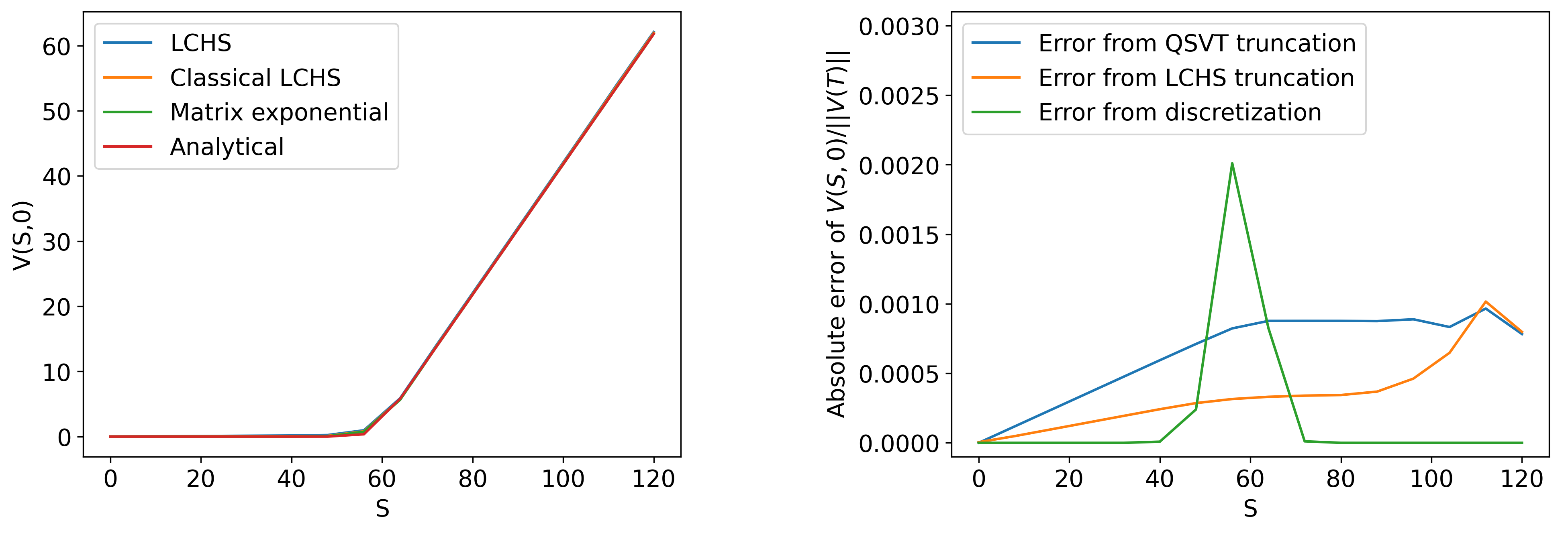
Figure 2: Numerical results for the one-asset Black–Scholes equation (left) and errors (right)

Next, Figure 3 shows the estimated number of Pauli rotation gates required and the number of logical qubits including auxiliary qubits, as functions of the number of grid points $N=2^n$ . As mentioned above, the theoretical order of the gate count is $O(2^{2n}n)$ ; for easier visual interpretation, $10\cdot 2^{2n}n$ is plotted in the figure. Although Encoding B requires more qubits than Encoding A, the gate count indeed appears to approach the theoretical order asymptotically.

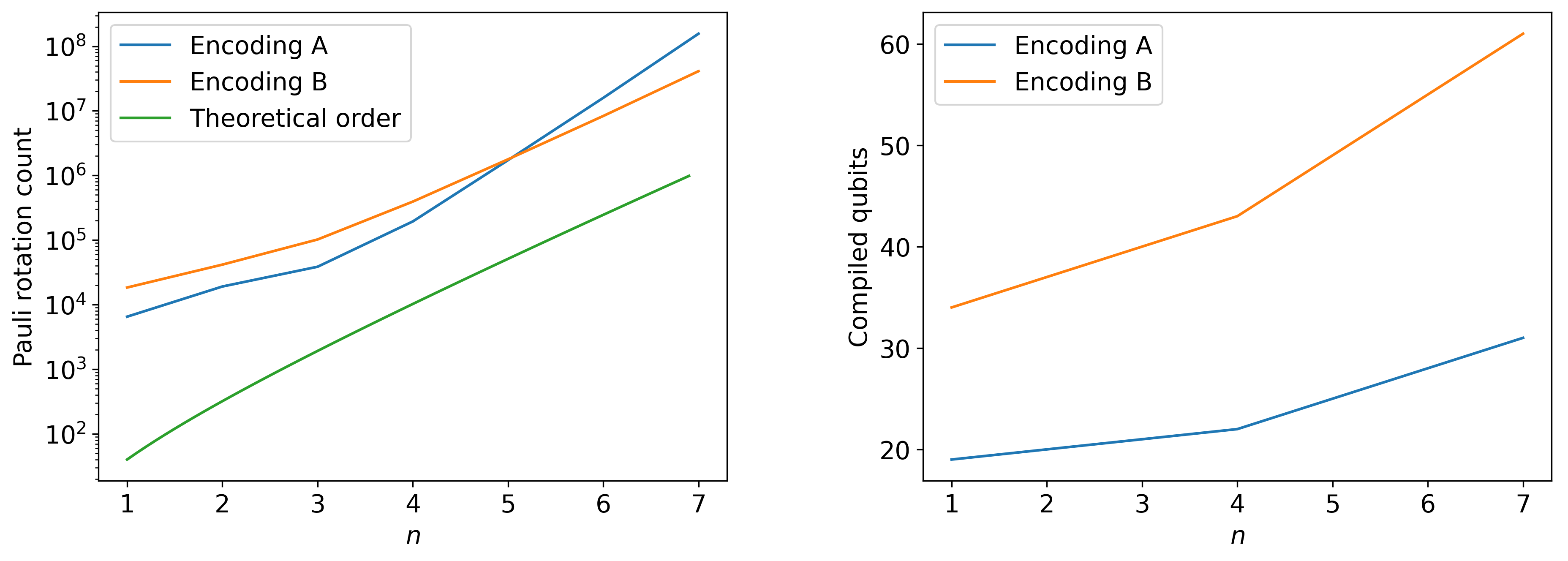
Figure 3: Number of Pauli rotation gates (left) and number of logical qubits after compilation (right)

Two-asset Black–Scholes equation

The same framework can also be extended to the multi-asset case. The two-asset Black–Scholes equation is:

\frac{\partial V}{\partial t} + \frac{1}{2} \sigma_1^2 S_1^2 \frac{\partial^2 V}{\partial S_1^2} + \rho \sigma_1 \sigma_2 S_1 S_2 \frac{\partial^2 V}{\partial S_1 \partial S_2} + \frac{1}{2} \sigma_2^2 S_2^2 \frac{\partial^2 V}{\partial S_2^2} + r S_1 \frac{\partial V}{\partial S_1} + r S_2 \frac{\partial V}{\partial S_2} - r V = 0

Here, $\sigma_i$ is the volatility of asset $i$ , $r$ is the risk-free interest rate, and $\rho$ is the correlation coefficient between the two assets. As the terminal condition, we adopt a worst-of call:

V(S_1,S_2,T)=\max(0,\min(S_1,S_2)-K)

The corresponding boundary conditions are:

V(0,S_2,t) = V(S_1,0,t) = 0 \,,\quad \lim_{S_1\to\infty} \partial_{S_1} V(S_1,S_2,t) = 0 \,,\quad \lim_{S_2\to\infty} \partial_{S_2} V(S_1,S_2,t) = 0

As in the one-asset case, if we discretize $S_1\in[0,S_{1,\max}]$ and $S_2\in[0,S_{2,\max}]$ into $N_1$ and $N_2$ points respectively, the price $V$ is represented as an $N_1N_2$ -dimensional vector. By applying central finite difference approximations and rearranging the coefficients, we obtain a homogeneous equation $d\vec{V}/dt=A\vec{V}$ , so we only need to compute $\vec{V}(0)=e^{-AT}\vec{V}(T)$ .

Figure 4 shows the results for parameters $S_{1,\max}=S_{2,\max}=120,K=40,\sigma_1=0.05,\sigma_2=0.02,r=0.03,\rho=0.4,N_1=N_2=2^2,T=1$ , with LCHS allowed error $\epsilon=0.1$ and QSVT allowed error $\epsilon_t=0.1$ . The characteristics of a worst-of call, whose value depends on the smaller underlying asset price, are visible. The right plot shows the number of Pauli rotation gates required for Encoding B as a function of grid points $N_1=2^{n_1}, N_2=2^{n_2}$ , together with a fit against $\alpha=\sigma_1^2N_1^2+\sigma_2^2N_2^2$ . The dominant order of the gate count is approximately $\alpha^{0.9}$ , which is consistent with the known theoretical order $O(N_1^2)+O(N_2^2)$ .

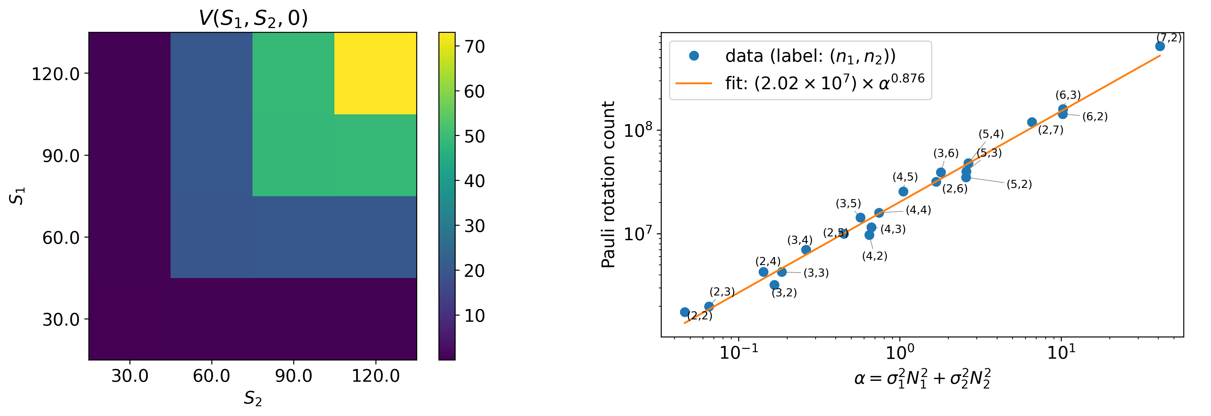
Figure 4: Numerical results for the two-asset Black–Scholes equation (left) and number of Pauli rotation gates (right)

Summary and future outlook

In this study, we implemented quantum circuits and performed simulations using LCHS for the problem of solving one-asset and two-asset Black–Scholes equations. We also varied the number of grid points used in the solution and estimated the required computational resources, including the number of non-Clifford gates and logical qubits.

Future work includes extending the approach to models that reflect more realistic markets, such as those with time-dependent interest rates and volatilities.

The resources estimated in this study assume an ideal quantum computer without considering error correction. Looking toward actual implementation on fault-tolerant quantum computers (FTQCs), it will be necessary to estimate physical qubit counts, gate counts, and execution time while taking encoding with quantum error-correcting codes such as the surface code into account. QURI SDK includes a feature called QURI VM, which performs compilation and resource estimation for surface-code-based architectures. Using QURI VM to evaluate resources in a form closer to actual hardware is an important direction for future work.

References

[1] N. Guseynov, N. Liu, C. S. Pun, T. Vaidya, “End-to-End PDE-Based Quantum Algorithms for Multi-Asset Option Pricing under Local and Stochastic Volatility,” arXiv:2605.26610 (2026).

[2] J. M. Martyn, Z. M. Rossi, A. K. Tan, I. L. Chuang, “Grand Unification of Quantum Algorithms,” PRX Quantum 2, 040203 (2021).

[3] G. H. Low, R. D. Somma, “Optimal quantum simulation of linear non-unitary dynamics,” arXiv:2508.19238 (2025).

[4] QunaSys Inc., https://quri-sdk.qunasys.com